Technology

History

Barcode Types

Barcode Printer

Inventory Management

Application

Software

Label Paper

Barcode Scanner

AI Barcode QRCode

Barcodes B

Barcodes C

Barcodes D

Barcodes E

Barcodes F

Robot Tech

Electronic

New Tech A

New Tech B

Psychology at Work

The most commonly used 10 Excel function formulas at work

SUM: The summation function:

Used to add numbers in a range of cells.

Syntax: =SUM(number1, [number2], ...).

For example, =SUM(A1:A5) will calculate the sum of the numbers in the range of cells A1 to A5.

AVERAGE: The average function:

Used to calculate the average of numbers in a range of cells.

Syntax: =AVERAGE(number1, [number2], ...).

For example, =AVERAGE(A1:A5) will calculate the average of the numbers in the range of cells A1 to A5.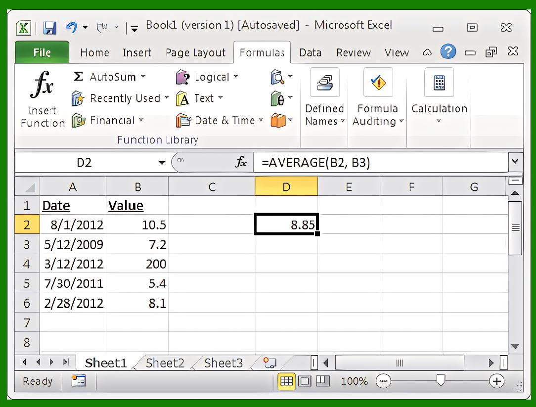

MAX: Maximum function:

Used to calculate the maximum value of numbers in a cell range.

Syntax: =MAX(number1, [number2], ...).

For example, =MAX(A1:A5) will calculate the maximum value of the number in the range of cells A1 to A5.

MIN: The Minimum function:

used to calculate the minimum value of numbers in a range of cells.

Syntax: =MIN(number1, [number2], ...).

For example, =MIN(A1:A5) will calculate the minimum value of the numbers in the range of cells A1 to A5.

COUNT: Counting function:

Used to count the number of numbers in a cell range.

Syntax: =COUNT(value1, [value2], ...).

For example, =COUNT(A1:A5) will count the number of numbers in the range of cells A1 to A5.

IF: Conditional function:

Used to return different results based on specified conditions.

Syntax: =IF(logical_test, value_if_true, value_if_false).

For example, =IF(A1>0, "Positive", "Negative") will return "Positive" or "Negative" based on the number in cell A1.

VLOOKUP: Vertical lookup function:

Used to find the specified value in the cell range and return the corresponding value.

Syntax: =VLOOKUP(lookup_value, table_array, col_index_num, [range_lookup]).

For example, =VLOOKUP(A1, B1:C5, 2, FALSE) will find the value in cell A1 in the range of cells B1 to C5 and return the corresponding second column value.

INDEX: Index function:

Used to return the value at the specified position within the cell range.

Syntax: =INDEX(array, row_num, [column_num]).

For example, =INDEX(A1:C5, 3, 2) will return the value in cell A3.

MATCH: The matching function:

Used to find the specified value within the cell range and return its position.

Syntax: =MATCH(lookup_value, lookup_array, [match_type]).

For example, =MATCH(A1, B1:B5, 0) will find the value in cell A1 in the range of cells B1 to B5 and return its position.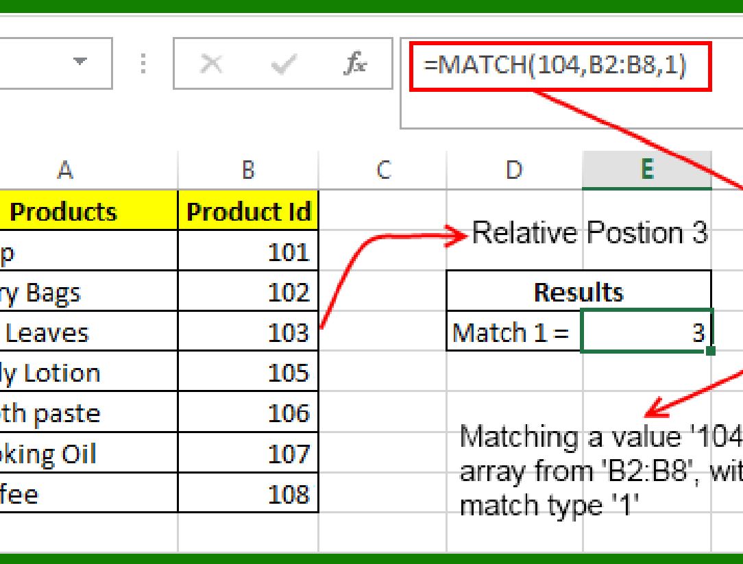

LEFT: Left function:

Used to return the specified number of characters on the left side of a text string.

Syntax: =LEFT(text, [num_chars]).

For example, =LEFT(A1, 3) will return the first three characters of the text string in cell A1.